Vignette for projecting data in the Stemformatics Integrated Atlas

Written by Jarny Choi. Last updated 11 November 2022

The Integrated Atlas page in Stemformatics provides a tool to project your own data, enabling a comparison of cell types in the data to those in the atlas. This vignette outlines how this can be done in detail with examples.

Citation

If you have found projecting your own data onto the Stemformatics atlas useful, please consider citing:
A simple, scalable approach to building a cross-platform transcriptome atlas, Paul W Angel, Nadia Rajab, Yidi Deng, Chris M Pacheco, Tyrone Chen, Kim-Anh Lê Cao, Jarny Choi, Christine A Wells, PLOS Comp Bio (2020), doi: https://doi.org/10.1371/journal.pcbi.1008219

Types of data and format

Since the atlas is currently built from microarray and bulk RNA-seq data, these are the primary data types the projection is currently designed for. The projection tool however does not discriminate on the source of data, as long as the row ids are Ensembl ids. Single cell RNA-seq data can be projected, but we have found that aggregating the data to simulate pseudo bulk data yields the best results (see example below or read Deng et.al. for an extended discussion). For microarray data, probe ids should be converted to gene ids before projecting.

The projection tool also requires a sample table, whose row ids match the columns of the expression matrix. Only one column from this table is required but having other columns allows you to view the projection results in different ways.

In summary, the projection tool requires 2 text files in tab separated format:

• An expression matrix with human Ensembl ids as row ids and sample ids as column names.
• A sample matrix with sample ids as row ids, matching the columns of the expression matrix (not necessarily in the same order). Only one column is required in this matrix but other columns can be useful.

During the projection, the input expression matrix will be filtered on genes which are present in the atlas, then rank transformed before projection is performed. If less than 50% of the genes in the atlas are present in the input matrix, the projection will not proceed and an error will result. The genes used by the atlas can be downloaded as a tab separated file from tools >> download data on the atlas page.

Example projection (bulk RNA-Seq)

In this example, we will project blood expression data onto the Stemformatics Blood Atlas and see if the projected samples are located close to the matching counterparts in the atlas on the PCA plot. Our input data come from haemosphere.org, which contains a selection of gene expression datasets specific to blood. In particular, we focus on Haemopedia-Human-RNASeq dataset, which contains samples from various blood lineages, including lymphocytes and myeloid cells.

The two files we need can be downloaded by clicking on the “download” button from haemosphere’s datasets page for Haemopedia-Human-RNASeq dataset. We can download “cpm values” and “sample table” files. Note that since these expression values will be rank transformed per sample independently of all other samples during the projection, the exact choice of normalisation used as input file is not so important.

# The downloaded expression matrix looks like this:
import pandas

hp = pandas.read_csv("Haemopedia-Human-RNASeq_cpm.txt", sep="\t", index_col=0)
display(hp.head())

	myDC123.2	myDC123.1	MonoNonClassic.1	CD4T.1	CD8T.1	Eo.1	myDC.1	MemB.1	Mono.1	NveB.1	...	NveB.4	NK.4	CD4T.5	CD8T.5	myDC.3	Mono.5	NveB.5	Neut.3	NK.5	pDC.2
genenames
ENSG00000223972	0.000000	0.000000	0.000000	0.000000	0.000000	0.00000	0.000000	0.000000	0.000000	0.000000	...	0.000000	0.000000	0.000000	0.000000	0.000000	0.000000	0.000000	0.000000	0.000000	0.000000
ENSG00000227232	1.224177	1.110908	4.317801	5.906965	2.579694	2.76102	1.205595	1.890113	3.837349	2.994901	...	2.893165	4.161794	5.296969	5.382940	5.235310	3.499009	4.533116	1.164611	4.606214	3.565716
ENSG00000278267	0.087441	0.000000	0.000000	0.000000	0.000000	0.00000	0.000000	0.000000	0.000000	0.000000	...	0.160731	0.189172	0.068792	0.139817	0.090264	0.000000	0.000000	0.000000	0.000000	0.075866
ENSG00000243485	0.000000	0.000000	0.000000	0.000000	0.000000	0.00000	0.000000	0.000000	0.000000	0.000000	...	0.000000	0.000000	0.000000	0.000000	0.000000	0.000000	0.000000	0.000000	0.000000	0.000000
ENSG00000274890	0.000000	0.000000	0.000000	0.000000	0.000000	0.00000	0.000000	0.000000	0.000000	0.000000	...	0.000000	0.000000	0.000000	0.000000	0.000000	0.000000	0.000000	0.000000	0.000000	0.000000

5 rows × 42 columns

# And the sample matrix looks like this
hpSamples = pandas.read_csv("Haemopedia-Human-RNASeq_samples.txt", sep="\t", index_col=0)
display(hpSamples.head())

	cellTypeAbbreviation	celltype	organism	long celltype	cell_lineage	immunophenotype	tissue	donor	totalReads	mappedPercent	assignedPercent
sampleId
MemB.1	MemB	Memory B Cell	Homo Sapiens	Memory B Cell	B Cell Lineage	CD3:- CD19:+ CD27:+	Peripheral Blood	Donor1	18699477	89.24	63.72
MemB.2	MemB	Memory B Cell	Homo Sapiens	Memory B Cell	B Cell Lineage	CD3:- CD19:+ CD27:+	Peripheral Blood	Donor2	17747099	89.89	60.29
MemB.3	MemB	Memory B Cell	Homo Sapiens	Memory B Cell	B Cell Lineage	CD3:- CD19:+ CD27:+	Peripheral Blood	Donor3	17434867	90.06	63.66
NveB.1	NveB	Naive B Cell	Homo Sapiens	Naive B Cell	B Cell Lineage	CD3:- CD19:+ CD27:-	Peripheral Blood	Donor1	18521249	90.24	59.43
NveB.2	NveB	Naive B Cell	Homo Sapiens	Naive B Cell	B Cell Lineage	CD3:- CD19:+ CD27:-	Peripheral Blood	Donor2	17695868	90.46	62.28

Note that even though row ids of the sample table should contain all column names of the expression matrix, they do not need to be in the same order.

Now we perform the projection using “Projection” >> “Project bulk data” function on the atlas page, where it asks to provide these two files, together with a name which will be used as a prefix to the projected samples for easier identification (we use “hp” as the name in this example). We also leave the sample column field blank here, which indicates we will use the first column of the sample table to group the projected samples together.

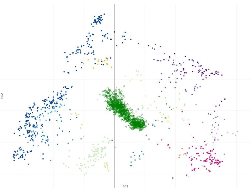
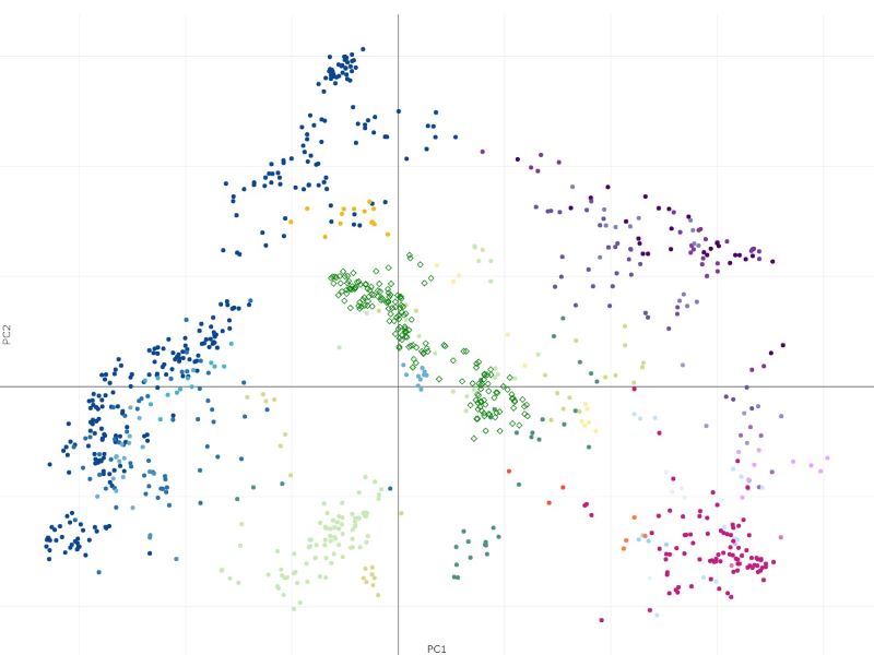
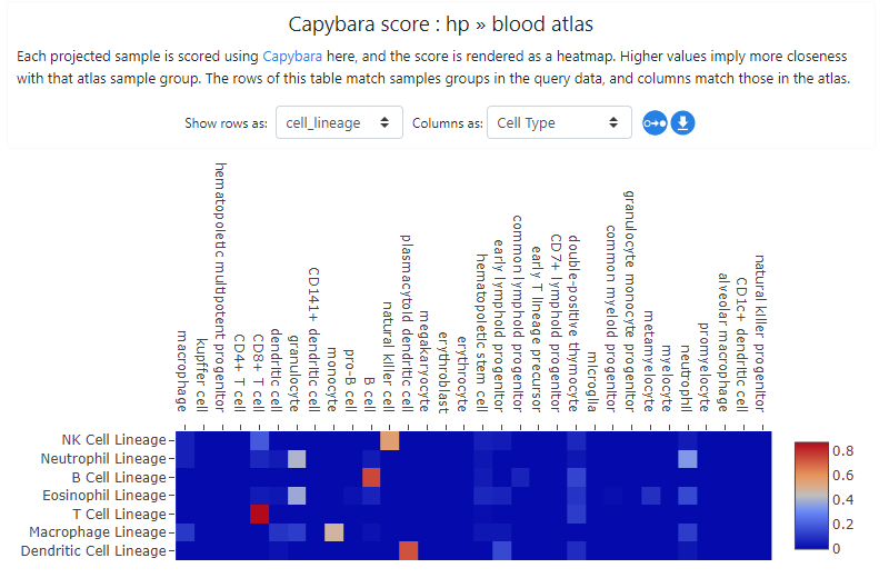
The projection process may take some time - it will scale with the expression file size being uploaded. The result is obtained as Capybara scores (Kong et.al.). In this example, the resulting projection shows a good biological concordance between the projected samples and cell types in the atlas, giving us some confidence that projection has worked well. Clicking on the "Show projections on PCA plot" button or simply going to Sample groups tab will also show the projected samples in the PCA space.

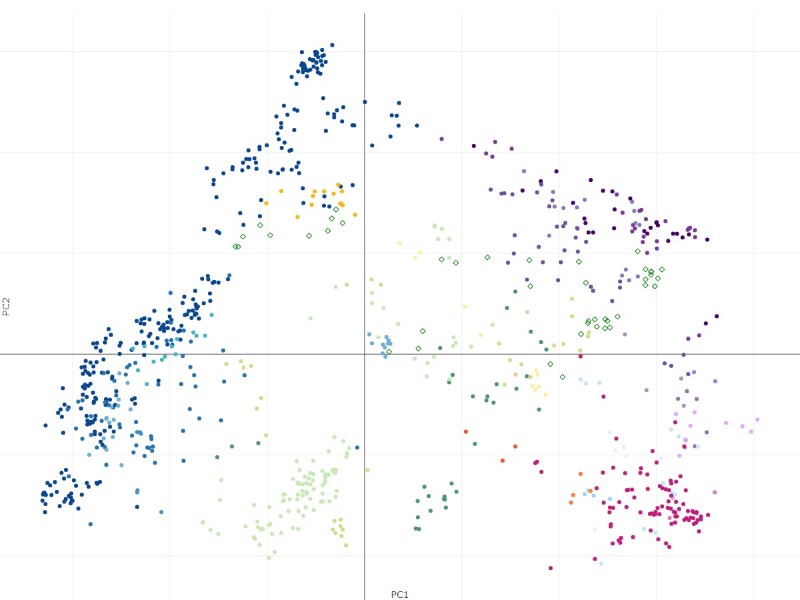
The samples from Haemopedia-Human-RNASeq data (diamond shapes) project onto the Stemformatics Blood Atlas near expected cell types. It is easier to see this by using the atlas page directly for projection using the files downloaded.

Projecting single cell data

Single cell RNA-seq data can be projected onto the atlas, but we have found that aggregating the data beforehand yields much better results than naively projecting each sample onto the atlas. This is due to the difference in the data structure between bulk and single cell RNA-seq data. There will also be performance issues for very large single cell datasets, both in terms of file upload and for processing if aggregation is not done.

As an example, we take this study by Villani, et. al. where they profiled human dendritic cells and monocytes to find sub clusters. We can download the files easily through the Broad Institute’s Single Cell Data Portal (note - you need to register and sign-in before downloading). We download “expression_matrix_tpm.txt” and “metadata.txt” files.

Note that the expression matrix here has gene symbols, rather than Ensembl gene ids, so we need to convert these first before projecting onto the atlas. There are various ways of obtaining the mapping between Ensembl gene ids to gene symbols, including using biomart or mygene.info. One simple option is to simply use the file provided on the atlas page :"Tools" >> "download data" >> "genes matrix", which contains this mapping.

# Read the downloaded expression matrix and samples files. Samples file has two rows of headers so we can skip one.
villani = pandas.read_csv("expression_matrix_tpm.txt", sep="\t", index_col=0)
villaniSamples = pandas.read_csv("metadata.txt", sep="\t", index_col=0, skiprows=1)

display(villani.head())
display(villaniSamples.head())

print("All columns of expression matrix are in samples:", set(villani.columns).issubset(set(villaniSamples.index)))

	CD141_P10_S73	CD141_P10_S74	CD141_P10_S75	CD141_P10_S76	CD141_P10_S77	CD141_P10_S78	CD141_P10_S79	CD141_P10_S80	CD141_P10_S81	CD141_P10_S82	...	Mono_nonclassical_S91	Mono_nonclassical_S92	Mono_nonclassical_S93	Mono_nonclassical_S94	Mono_nonclassical_S95	Mono_nonclassical_S96	Mono_nonclassical_S97	Mono_nonclassical_S98	Mono_nonclassical_S99	Mono_nonclassical_S9
GENE
1/2-SBSRNA4	0.000000	0.0	0.0	0.0	1.208960	1.853168	1.261298	0.000000	0.667829	0.0	...	1.534714	0.0	0.000000	0.0	0.0	0.936093	0.00000	0.000000	0.00000	0.0
5S_RRNA	0.000000	0.0	0.0	0.0	0.000000	0.000000	0.000000	3.029650	0.000000	0.0	...	0.000000	0.0	0.000000	0.0	0.0	0.000000	0.00000	0.000000	0.00000	0.0
5_8S_RRNA	0.000000	0.0	0.0	0.0	0.000000	0.000000	4.152456	0.000000	0.000000	0.0	...	0.000000	0.0	0.000000	0.0	0.0	0.000000	0.00000	0.000000	0.00000	0.0
7SK	4.625365	0.0	0.0	0.0	4.549975	0.000000	3.035434	2.436241	0.000000	0.0	...	0.000000	0.0	2.978077	0.0	0.0	3.355502	3.64545	3.844814	3.78646	0.0
A1BG	2.670694	0.0	0.0	0.0	0.000000	0.000000	0.000000	0.000000	0.000000	0.0	...	0.000000	0.0	0.000000	0.0	0.0	0.000000	0.00000	0.000000	0.00000	0.0

5 rows × 1078 columns

	group
TYPE
CD141_P10_S73	DC1
CD141_P10_S74	DC5
CD141_P10_S75	DC1
CD141_P10_S76	DC1
CD141_P10_S77	DC1

All columns of expression matrix are in samples: True

Even though we will aggregate the samples before projecting, we can see what happens first without any aggregation as a comparison. So first convert the gene symbols to Ensembl ids and save this file. Also remove one extra row of headers from sample table as that won't work for projection.

"""
Function to convert row ids in pandas DataFrame df from gene symbols to Ensembl gene ids.
Uses the gene annotation file downloaded from Stemformatics atlas page.
"""
def convertGeneSymbolsToEnsemblIds(df, geneAnnotationFile="blood_atlas_genes_v7.1.tsv"):
    genes = pandas.read_csv(geneAnnotationFile, sep="\t").set_index("symbol")
    commonSymbols = list(set(genes.index).intersection(set(df.index)))

    # drop duplicate index from expression before running reindex
    df = df.loc[~df.index.duplicated(keep='first')].reindex(commonSymbols)
    df.index = genes.loc[commonSymbols]["ensembl"]
    return df

# Use the function to save Ensembl id version of villani data. Also save sample table with fixed headers.
convertGeneSymbolsToEnsemblIds(villani).to_csv("expression_matrix_tpm_EnsemblIds.txt", sep="\t")
villaniSamples.to_csv("metadata_fixed_header.txt", sep="\t")

When we project this unaggregated data directly onto the atlas, the projected samples tend to cluster together rather than show sufficient similarity with atlas cell types to make inferences.

Now we aggregate based on the clusters which are already assigned by the second column of metadata.txt file. The number of individual samples to aggregate within a cluster can be determined in various ways, but we have found that aggregating between 5-8 cells is sufficient to approximate the distribution of bulk data. More details on this can be found in Rajab et.al. (See supplementary methods where it talks about using Kolmogorov–Smirnov statistic to work out the optimal aggregation size using this same dataset). Or for a full discussion and options on how best to project single cell data onto our atlases, see Deng et.al..

"""
Function to gggregate pandas DataFrame df and return the aggregated data frame and a matching sample table.
    Example: dfNew, samplesNew = aggregateExpressionMatrix(df, ["HSC","Mono","HSC",...])
groups is a list of sample group items, same length as columns of df, denoting which sample belongs to which group.
size is the number of samples in each group to sum over - random selection with replacement will be used.
"""
import numpy

def aggregateExpressionMatrix(df, groups, size=6):
    
    # Convert the list into pandas Series to take advantage of its features
    groups = pandas.Series(groups)
    
    # Aggregated data frame and new sample group membership to return
    aggregated = pandas.DataFrame()
    aggSampleGroup = []
    
    for group in groups.unique():  # loop through each unique item in groups
        
        # Indices of groups which match this group
        matchingIndex = groups[groups==group].index
        
        # How many aggregated samples should we produce per group? 
        # Here we divide number of samples in the group by size. Take size if this number is smaller.
        numberOfSamples = max(round(len(matchingIndex)/size), size)
                
        for i in range(numberOfSamples):
            # Select a subset of matchinIndex randomly with replacement. So chosenIndex may have duplicates.
            chosenIndex = numpy.random.choice(matchingIndex, size)

            # new sample id
            sampleId = "%s_%s" % (group, i)
            aggSampleGroup.append([sampleId, group])
            
            # Construct a column "subset" of df using chosenIndex, where duplicates may be present,
            # then sum these column-wise and add this to aggregated
            subset = df.iloc[:,chosenIndex]
            aggregated[sampleId] = subset.sum(axis=1)
        
    return aggregated, pandas.DataFrame(aggSampleGroup, columns=['sampleId', 'group']).set_index('sampleId')
    
villaniAggregated, villaniAggSamples = aggregateExpressionMatrix(villani, villaniSamples["group"].tolist())
print(villaniAggregated.shape)
display(villaniAggregated.head())

(26593, 185)

	DC1_0	DC1_1	DC1_2	DC1_3	DC1_4	DC1_5	DC1_6	DC1_7	DC1_8	DC1_9	...	DC6_25	DC6_26	DC6_27	DC6_28	Mono3_0	Mono3_1	Mono3_2	Mono3_3	Mono3_4	Mono3_5
GENE
1/2-SBSRNA4	5.651161	2.032088	1.885553	8.382685	3.210061	3.040054	5.545655	7.718105	8.314636	5.579928	...	5.998881	4.023385	0.916291	0.000000	4.949551	7.380411	0.000000	0.000000	3.249040	3.85469
5S_RRNA	0.000000	4.044279	4.477564	0.000000	0.000000	3.291010	0.000000	0.000000	0.000000	4.044279	...	0.000000	0.000000	0.000000	0.000000	0.000000	0.000000	0.000000	5.057964	0.000000	0.00000
5_8S_RRNA	0.000000	0.000000	0.000000	4.183728	0.000000	0.000000	0.000000	0.000000	0.000000	0.000000	...	0.000000	0.000000	0.000000	0.000000	0.000000	0.000000	0.000000	0.000000	0.000000	0.00000
7SK	11.921593	3.379633	4.850858	16.950666	4.942071	7.402615	9.517593	8.238556	2.282382	8.538484	...	0.000000	3.517498	7.053788	4.795046	12.975854	4.965568	7.102106	3.789177	14.023648	0.00000
A1BG	1.633154	0.000000	4.091674	2.070653	0.285179	0.000000	0.000000	2.070653	5.439958	0.000000	...	0.000000	7.401218	0.000000	3.787763	3.281663	3.281663	4.783023	3.281663	4.621107	0.00000

5 rows × 185 columns

# Convert aggregated matrix to use Ensembl ids. We didn't do this before aggregation since some genes will drop out 
# in the process of mapping to gene ids, and we want to keep as many genes as we can during the aggregation process.
villaniAggregated = convertGeneSymbolsToEnsemblIds(villaniAggregated)
display(villaniAggregated.head())

	DC1_0	DC1_1	DC1_2	DC1_3	DC1_4	DC1_5	DC1_6	DC1_7	DC1_8	DC1_9	...	DC6_25	DC6_26	DC6_27	DC6_28	Mono3_0	Mono3_1	Mono3_2	Mono3_3	Mono3_4	Mono3_5
ensembl
ENSG00000116698	1.047319	8.749755	1.388791	5.990058	3.913622	6.092775	0.000000	5.319374	1.169381	0.000000	...	7.452496	7.715534	8.329410	3.704871	13.112474	14.401569	19.347299	12.298960	7.207455	16.023954
ENSG00000088205	16.607080	7.829327	12.671372	15.057319	8.433056	13.987898	5.140628	11.858718	9.835893	8.760485	...	24.938408	16.630552	9.860245	5.396706	16.807234	12.230230	1.701105	12.272025	15.599035	3.936638
ENSG00000077327	2.215948	0.000000	0.000000	1.841660	0.536493	1.249988	1.268861	0.978326	4.281652	1.121678	...	0.000000	0.000000	0.000000	0.000000	2.303744	3.050629	3.961448	1.371181	3.603027	2.749960
ENSG00000091039	12.078762	8.438128	11.947039	16.719615	7.717399	10.034621	6.374665	9.214563	6.977688	17.548167	...	21.513627	14.539010	16.512262	9.797026	18.231193	27.684564	21.584457	23.469503	15.274974	21.452959
ENSG00000118503	5.951538	4.904341	7.379061	6.794721	8.898817	2.656055	3.021186	4.634719	3.621612	7.817818	...	17.674313	12.440998	10.070372	13.044396	19.345186	19.756043	22.068908	15.281602	22.501590	12.960494

5 rows × 185 columns

# We can now write this aggregated matrix to file, together with new sample table
villaniAggregated.to_csv("villani_aggregated_expression.tsv", sep="\t")
villaniAggSamples.to_csv("villani_aggregated_samples.tsv", sep="\t")

Using these files now for projection yields a better result.

The samples from Villani data after aggregation (diamond shapes) project onto the Stemformatics Blood Atlas. It is easier to explore this on the web page directly after projection. This plot is provided here for a quick reference.

Interpreting the projection and limitations

Projections show the transcriptional similarity between atlas samples and projected samples using the Capybara method and within the PCA framework. Hence if a projected sample is close to an atlas sample in the PCA plot, it indicates that genes in the atlas with high loadings for the first few principal components share a similar expression pattern in the projected sample after a rank transformation. Note that if a sample is very different to all the samples in the atlas, it will tend to sit in the middle of the plot. This is usually what happens when we project single cell RNA-seq data without any aggregation, due to its very different data structure.